GIS Portfolio: Ross Wygmans

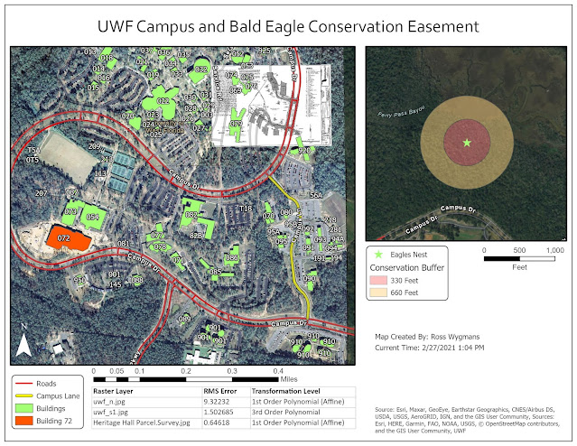
  This weeks lab introduced us to the concept of georeferencing, which essentially means taking a raster dataset (such as an aerial image) with no coordinate information and aligning it in the correct place. Georeferencing is particularly helpful when working with datasets created prior to the widespread use of GIS, such as scans of old surveys or paper maps. We also learned how to create new polygon and line features within a vector layer.  In the second portion of the lab, we used LIDAR data to create a 3D map of the University of West Florida main campus. The LIDAR data was first converted to an elevation raster layer and then the aerial images were draped over the top top of the elevation layer.  

  Sometimes, the only spatial data available may be in the form of street addresses. In this case, we can use the Geocode feature in ArcGIS Pro to match addresses to a horizontal coordinate system. Address information for schools in Brevard County, Florida were copied from the Florida Department of Education website. These addresses were then matched to an edges (streets) layer downloaded from the US Census Bureau Geography Program using a customized Address Locator created in ArcGIS Pro. Although the Geocode feature can be quite effective, there will almost always be some addresses that cannot be matched properly. In this case, I used Google Maps to find the location of unmatched schools and the Pick From Map option within ArcGIS Pro to match the schools using the aerial imagery.   You can access my web map  here . 

  Have you ever tried to find that perfect camping spot? In this assignment, we were asked to locate possible campsites within the De Soto National Forest near Hattiesburg, Mississippi. These sites had to be within 300m of existing roads, within 500m of rivers or 150m of lakes, and could not be located within existing conservation areas.   To accomplish this task, we used three primary geoprocessing tools: Buffer, Union, and Erase. The roads layer was buffered to 300m using a fixed distance buffer, and the rivers and lakes were buffered to 500m and 150m respectively using a variable distance buffer. These two buffered layers were then overlaid using the Union tool to locate all the areas that fell within both the roads buffered layer and and the water buffered layer. Areas that fell within conservation areas were then excluded using the Erase tool. Finally, the campsites polygons were ranked into three different classes (Good, Better, and Best) based on the size of each polygon, with l

  This week's lab highlighted small discrepancies that can occur when using various map projections that may lead to significant errors when performing spatial analysis. This map shows the state of Florida using three different projections: Albers Conical Equal Area, UTM Zone 16N, and Florida State Plane North. While visual differences between the three map frames may be negligible, the table displays the area in square miles for each of the four selected counties that were calculated using these different projections.